Neural Operators (Kovachki et al. 2022) and Fourier Neural Operator (Li et al. 2021) papers were presented by Michael Innerberger and Magdalena Schneider in Janelia CVML 2024-11-01 (and discussed in this blog post), Adaptive Fourier Neural Operator (Guibas et al. 2022) and FourCastNet (Pathak et al. 2022) papers were presented by Magdalena Schneider and Kristin Branson in Janelia CVML 2024-11-08 (see blog post on FourCastNet)
Neural Operators extend the concept of neural networks to work directly with functions rather than discrete data points. While neural networks typically take vectors or tensors as inputs and produce similar outputs, Neural Operators learn mappings between entire functions. A major advantage of neural operators is their (presumed) discretization invariance, which allows for zero-shot super resolution, meaning that the output function can be evaluated at an arbitrary set of query points without the need to retrain the neural operator. Originally developed for solving PDEs, neural operators have been successfully applied to a wide range of problems, including computer vision tasks. In this blog post, we will introduce the concept of neural operators, discuss different ways to represent the kernel, and present some hands-on examples.
We assume that you are familiar with some fundamental concepts of vector calculus like partial derivatives of multi-variate functions. Some background in Partial Differential Equations (PDEs) and fundamental solutions to PDEs would be ideal as this is the theoretical foundation of Neural Operators, but not strictly necessary.
What are Neural Operators?
Conventional neural networks have finite-dimensional inputs and outputs, which are represented as vectors. However, many real-world problems are continuous in nature and better represented by a function. Neural Operators are a generalization of neural networks that can learn to map functions to functions. They can be used to solve PDEs, inverse problems, and other tasks that involve finding functions defined over continuous domains. Neural operators can also be applied to learn mappings between neural representations, as neural representations are function representations.

Motivation
The main motivation behind Neural Operators is that some linear PDEs of the form \(\mathsf{L}_a u = f\) with parameter functions \(a \colon D \to \mathbb{R}^m\) in some domain \(D \subset \mathbb{R}^d\) and source term \(f\) can be solved by convolution with a fundamental solution \(k\) of the PDE. Note that either the source term \(f\) or the parameter function \(a\) can be fixed, and the other is the input to the solution operator which gives us \(u\). If we want to find the solution for varying \(f\), the solution operator \(G \colon f \mapsto u\) mapping a given source term \(f\) to the solution \(u\) is given by \[ u(x) = \int_D k(x, y) f(y) \, dy. \tag{1}\] While this is only possible for a small set of very specific PDEs, this representation of the solution serves as a basic building block for neural operators, on top of which a deep learning architecture is built. We stress that Equation 1 is only a motivation and not a theoretical justification for why neural operators work. In particular, neural operators can be applied to a much wider range of problems such as non-linear PDEs and inverse problems; in particular, in the following, we consider the case where the source term \(f\) is fixed and the Neural Operator learns to map a parameter function \(a\) to the solution \(u\).
Illustrative example
To illustrate the concept of how Neural Operators solve PDEs, we will consider a simple example of a PDE and return to this example throughout the text to explain the different concepts. The physical model for the Darcy flow is a relatively simple PDE that describes the flow of a fluid through a porous medium (e.g., water through sand). In its two-dimensional form on the unit square \(D = [0, 1]^2\), the Darcy flow equation is given by \[ -\nabla \cdot (a(x) \nabla u(x)) = f(x), \] where \(u(x)\) is the pressure of the fluid, \(a(x)\) is the local permeability of the medium, and \(f(x)\) is an external source term modeling fluid entering or leaving the system. Without porous medium, fluid flow is given by the pressure gradient \(\nabla u\), so \(a(x)\) intuitively acts as a local modifier of the driving force behind the flow. The quantity \(a(x) \nabla u(x)\) is called the flux of the fluid, and the Darcy flow equation states that the sources (which are given by the divergence operator \(\nabla \cdot\)) of the fluid flux are given by \(f\).
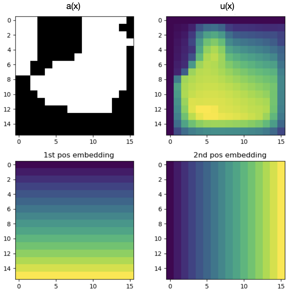
Fixing the source term \(f(x) = 1\) and the boundary condition \(u(x) = 0\) (meaning that there is no fluid pressure) on the boundary \(\partial D\), the problem is to find the pressure field \(u(x)\) for a given permeability field \(a(x)\). Pairs of \(a(x)\) and \(u(x)\) are shown in Figure 9, where the input function \(a(x)\) is shown on the left as a binary scalar field over the unit square, and the corresponding output function \(u(x)\) is shown on the right, having a more intricate structure. Note that the images shown in the figure are just discrete representations of the functions \(a(x)\) and \(u(x)\) defined on the whole domain \(D\), which are the input and output of the PDE problem (and the Neural Operator).
In the context of Neural Operators, the goal is to learn the inverse \(\mathsf{L}_a^{-1}f\) of the differential operator \(\mathsf{L}_a = -\nabla \cdot (a(x) \nabla (\cdot))\), which maps the parameter function \(a(x)\) to the solution \(u(x)\). Note that the Darcy flow with a general permeability field \(a(x)\) doesn’t have an analytically known fundamental solution, and the mapping from \(a(x)\) to \(u(x)\) is highly non-linear, so that in order to solve the PDE numerical or machine learning methods are necessary, such as Neural Operators.
General architecture
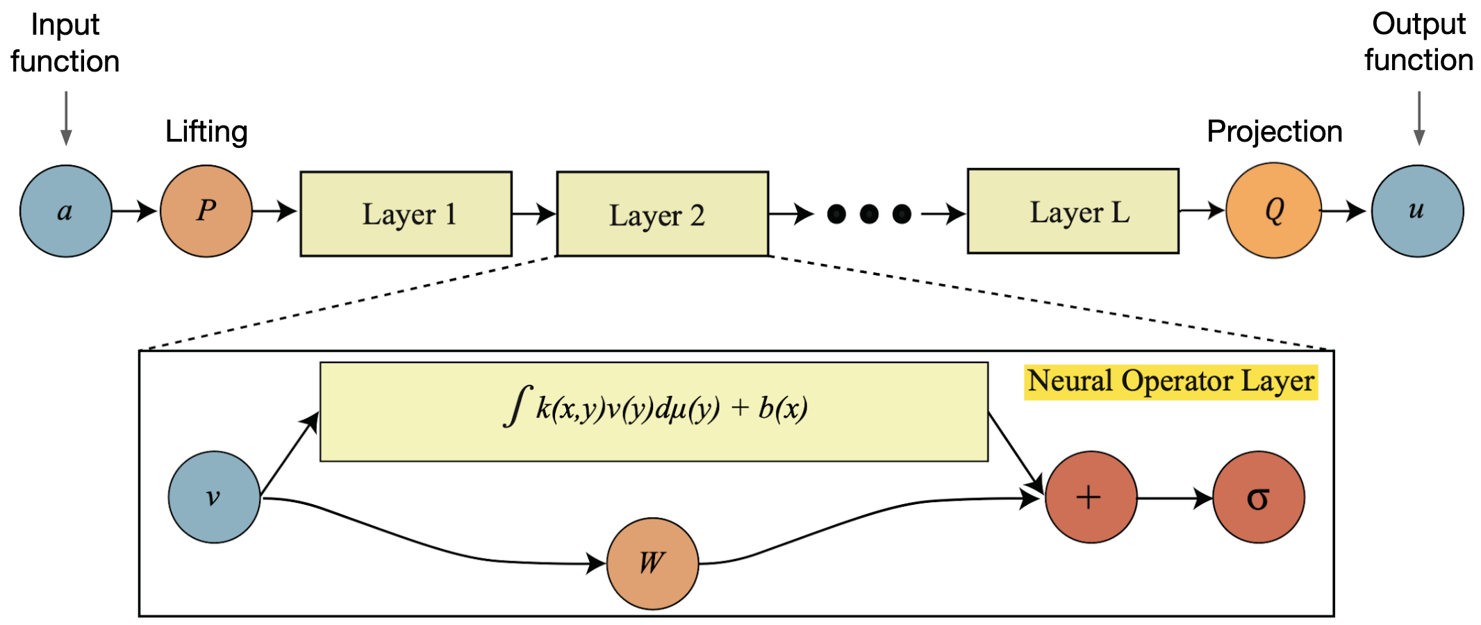
Put simply, Neural Operators can be seen as a generalization of convolutional neural networks (CNNs) to continuous domains. While CNNs feature convolutions with small kernels on regular discrete grids, neural operators have a continuous kernel that is convolved with the whole function in each layer. The general architecture of a Neural Operator is shown in Figure 2. The input function \(a\) (usually represented by a set of query points and corresponding function values—see Section 1.4) is lifted into a (usually higher-dimensional) space by \(P\). Then, the lifted function is processed by a series of layers, each of which applies a convolution with a continuous kernel to the function. The resulting function is added to a linear term \(W v\) and then passed through a non-linear activation function; note that this is akin to a skip connection in a CNN. Finally, the result of this computation is projected to the output space by the projection \(Q\), yielding the output function \(u\). Note that the output function can be queried at any point in the domain, which is a key feature of Neural Operators.
Discretization and invariance
Although Neural Operators are designed to learn mappings between functions on continuous domains, for numerical implementation, the functions still needs to be discretized, i.e., represented by a set of query points and corresponding function values \(\{x_i, a(x_i)\}_i\). The query points of \(u(x)\) are supplied together with the input function, as they need to pass through the whole network. While, in principle, the query points can be arbitrary, in practice they are often chosen to be equidistantly spaced on a grid for computational efficiency. Hence, the true learned operator \(\widehat{G} \colon a \mapsto u\) (operating on functions) is approximated by the discretized operator \(\widehat{G}_L\), operating on \[ \widehat{G}_L \colon \mathbb{R}^{L \cdot m} \times \mathbb{R}^{L \cdot d} \rightarrow \mathcal{U}, \] where \(L\) is the number of query points of the input function, \(d\) and \(m\) are the dimensions of the domain \(D\) and the image of the input function, respectively, and \(\mathcal{U}\) is the function space of the output function. Notably, the output function \(u(x)\) can be evaluated at any set of query points, which do not have to be the same as the query points of the input function, or the query points used for training. This allows for “zero-shot super resolution”, i.e., the output function can be evaluated at arbitrarily high resolution without the need to retrain the neural operator at different resolutions.
Discretization invariance refers to the fact that \(\widehat{G}_L\) converges to \(\widehat{G}\) as \(L \to \infty\) (under some mild conditions to the distribution of the query points). Again, increasing \(L\) does not require retraining the Neural Operator. Note that some other papers have claimed that Neural Operators are not necessarily discretization invariant (e.g., Wang and Golland (2023)); this is a topic of ongoing research.
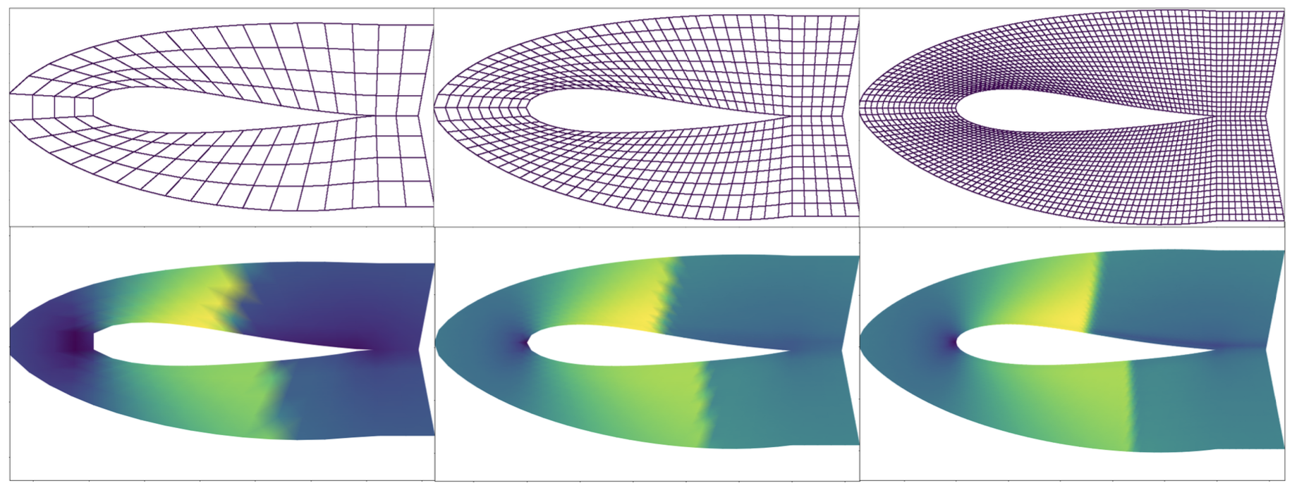
In our example of the Darcy flow from Section 1.2 and Figure 9, the input function \(a(x)\) is discretized on a grid of \(L = 16 \times 16 = 256\) query points, resulting in a matrix with \(256\) rows of the form \(\{x_{i,1}, x_{i,2}, a(x_{i})\}\) being supplied to the Neural Operator. Each row is mapped to a positional embedding by the projection \(P\), and the results are used as values \(v(y)\) in the convolution operation. In order to evaluate the output function \(u\) at a point \(z \in D\), the query point \(z\) is supplied to the Neural Operator together with point evaluations of the input function \(a(x)\) to obtain an output value \(u(y)\). Since this can be done for any point \(z\), the output of the Neural Operator is a proper function (meaning infinite resolution), while the input is still a set of query points and function values. If more sampling points of the input function are supplied, discretization invariance ensures that the output function becomes more accurate, converging to the true solution (where the input is the full function \(a\)) as the number \(L\) of query points goes to infinity. Notably, this doesn’t require retraining the Neural Operator.
Different ways to represent the kernel
The bottleneck of Neural Operators is the convolution operation, the cost of which scales with the product of input and output size. Assuming that input and output are queried at the same \(L\) points, the complexity of the convolution is \(\mathcal{O}(L^2)\), which is infeasible for most applications. Fortunately, there are multiple ways to speed up the computation of the convolution based on the structure of the kernel, which we will shortly describe in the following (for details see Kovachki et al. (2022)).
Graph Neural Operators
Instead of taking into account the full space of pairs of sample points, we can limit the evaluation of the kernel to pairs of points that are close to each other. In practice, this can be done by constructing a graph that connects points that are within a certain distance of each other by using a nearest neighbor search. It is then advantageous to use graph neural networks to compute the convolution operation on this graph structure, and to be able to backpropagate easily through this operation. This reduces the complexity to \(\mathcal{O}(kL)\), where \(k\) is the maximal number of neighbors within a specified distance. Note that \(k\) can, in general, not be chosen independently of \(L\) (the number of query points of the input function) as \(L\) increases.

Multipole Graph Neural Operators
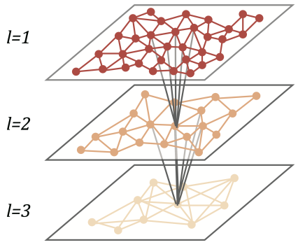
Graph Neural Operators only take nearest neighbor interactions into account. While this might be sufficient for some applications, long-range interactions also play a crucial role in many real-world problems (e.g., celestial mechanics, or electrodynamics). Drawing from ideas of the fast multipole method (FMM) presented in Greengard and Rokhlin (1987), Multipole Graph Neural Operators (MGNOs) use a hierarchical sequence of graphs to approximate the convolution operation. Every node in one of these graphs summarizes the information of a group of nodes in the previous hierarchy level as shown in Figure 5, and every level of the hierarchy gives rise to a certain scale-dependent component of the kernel. While the details are complex, the idea is similar to enlarging the context window of a CNN by using a sequence of convolutional layers with small kernel sizes. This reduces the complexity to \(\mathcal{O}(L)\).
Low-rank Neural Operators
By assuming that the kernel can be approximated by a low-rank factorization, \[k(x, y) \approx \sum_{i=1}^r \varphi_i(x) \varphi_i(y),\] with learnable functions \(\varphi_i \colon D \to \mathbb{R}\), and \(r \ll L\), the convolution operation can be computed in \(\mathcal{O}(rL)\). While this can significantly reduce the computational cost, it is important to note that the low-rank assumption might not hold for all problems and that the choice of low-rank approximation (i.e., the functions \(\varphi\)) can be crucial but non-trivial.

Fourier Neural Operators
Fourier Neural Operators (FNOs) are based on the Fourier representation of the convolution operation: \[\int_D k(x, y) v(y) \, dy = \mathcal{F}^{-1}(\mathcal{F}(k) \odot \mathcal{F}(v)),\] where \(\mathcal{F}\) is the Fourier transform, and \(\odot\) denotes the element-wise vector or matrix product. In practice, this seems to give the best results and can be combined with low-pass filtering to reduce the computational cost even further; see Figure 7, where the Fourier representation \(R\) of the kernel is learned and only low frequencies are propagated through the network.
While, in general, computing the Fourier transform scales quadratically with the input size, the fast Fourier transform (FFT) can be used to compute it in almost linear time if the input grid is uniform on a periodic domain (which by embedding the domain \(D\) in a larger domain and extending the input function by zero padding can be achieved for many applications). In this case, the complexity of the convolution operation is \(\mathcal{O}(L \log L)\).

Practical examples
Kovachki et al. (2022) provides various examples of solving PDEs with Neural Operators. We picked three examples here that (i) compare the performance of neural operators to the analytic solution, (ii) show a simple example that you can train yourself with code provided by the authors, and (iii) demonstrate how Neural Operators can solve inverse problems much faster than classical methods.
Note that, in order to generate training data, in Kovachki et al. (2022) the PDEs were solved with classical numerical methods, such as finite differences, finite elements, or spectral methods; see, e.g., Bartels (2018). Of note, all of these methods require knowledge of the PDE that models the physical phenomenon of interest, and they take significant resources to implement and compute the solution. While using data from classical methods to train is one common approach, it is also possible to train neural operators directly from data, which was done, for example, in the FourCastNet paper (Pathak et al. 2022), and is an active area of research.
Poisson equation: compare fundamental solutions
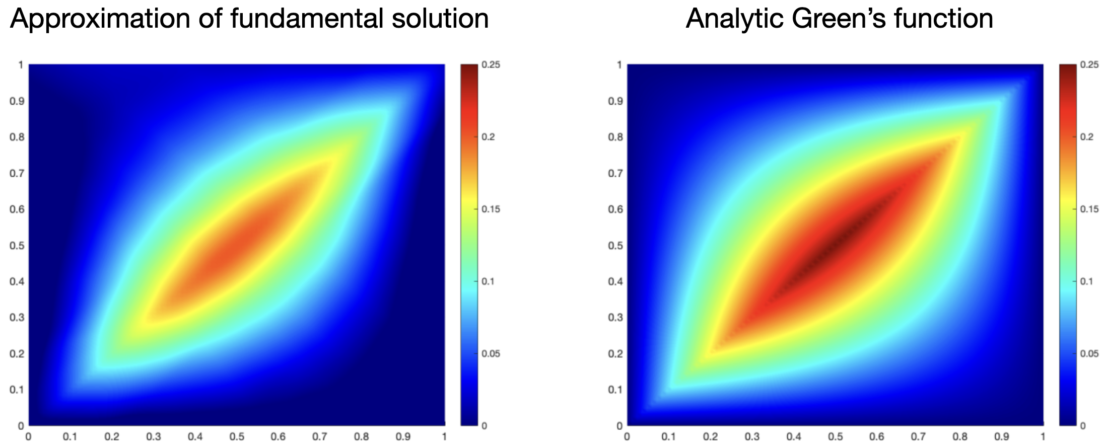
The Poisson equation is a fairly simple PDE that has an analytical solution. We can use this to check how well the Neural Operator approximates the ground truth. The Poisson equation is given by \[ -\frac{\partial^2 u}{\partial x^2} = f(x), \quad x \in (0, 1), \] with boundary conditions \(u(0) = u(1) = 0\). The fundamental solution (also called Green’s function) is given by \[ k(x, y) = \frac{1}{2}(x+y - |y-x|) - xy, \] so the solution for any \(f\) is given by \[ u(x) = \int_0^1 k(x, y) f(y) \, dy. \] Note that—as pointed out previously—a fundamental solution does not exist for every PDE—only a subset of linear PDEs with appropriate boundary conditions have one. A full Neural Operator architecture has several layers and thus, we don’t usually have a direct representation of the fundamental solution, either. This simple example of a Poisson equation was trained with a single layer, no bias and linear skip connection, and identity activation, so that the learned kernel is directly interpretable as the fundamental solution and can be compared to the ground truth. Figure 8 shows both the analytic fundamental solution and the learned kernel. Of note, they are not exactly the same, but qualitatively similar, which gives rise to the good generalization properties when querying the output function at arbitrary points.
Darcy flow: train a simple Neural Operator yourself
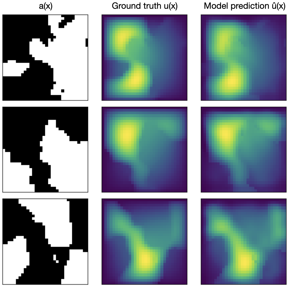
We again turn to the Darcy flow problem from Section 1.2. Figure 9 (a) shows an illustrative training dataset for the Darcy flow problem including the input function, output function and positional embedding. Figure 9 (b) shows the prediction of the trained Neural Operator for three different input functions \(a(x)\), and ground truth for comparison. The shown examples were reproduced by code provided by the authors (see resources for links). They were trained on a \(16 \times 16\) grid, which requires minimal computation, so you can easily train them yourself on a standard cpu.
Note that this example actually uses a slightly adapted version of the training process, where both trained frequencies and the resolution of the input data are increased incrementally. The Incremental Fourier Neural Operator (iFNO) was introduced in George et al. (2022).
Inverse problems: solve them much faster than classical methods
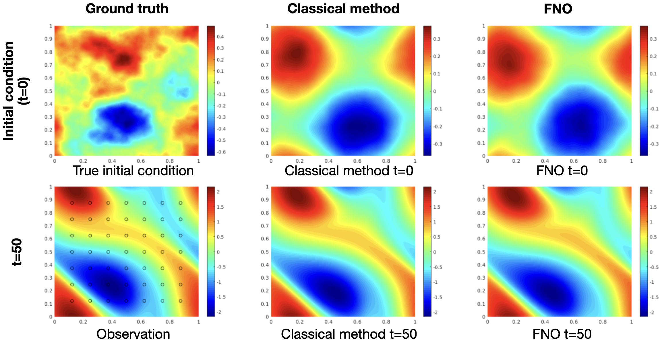
Neural Operators can also be applied to efficiently solve Bayesian inverse problems, where the goal is to recover the initial condition or coefficient functions of a PDE from noisy observations. Here, we look at a simulation of a two-dimensional viscous, incompressible fluid flow governed by the Navier–Stokes equations in their vorticity-streamfunction formulation. We’ll skip the details of the PDE and just note the general setup: Figure 10 (left column) shows the initial condition at timepoint \(t=0\) and the corresponding state at timepoint \(t=50\). The goal is to recover the initial condition from sampling the state at timepoint \(t=50\) which is affected by noise.
For solving the inverse problem for a single state, a classical method (middle column) based on spectral methods took 18 hours to compute the solution (Kovachki et al. 2022).
Meanwhile, a Fourier Neural Operator (FNO) for solving the inverse problem can be trained on training data pairs obtained by forward simulation using classical methods. After training of the Neural Operator, which took 12 hours (including generation of training data), solving the inverse problem for each new single state takes only 2.5 minutes (right column), making this approach much more efficient than solving the whole inverse problem with classical methods.
Applications in computer vision
Neural Operators have been successfully applied to real-world problems, including weather forecasting (Pathak et al. 2022) (see also our blog post on FourCastNet) and CO2 storage (Wen et al. 2023).
Moreover, Neural Operator learning is not restricted to PDEs, but can also be applied to computer vision tasks: images can naturally be viewed as real-valued function on 2D domains, and videos add a temporal structure. Examples of computer vision tasks that have been successfully tackled with Neural Operators include image inpainting, super-resolution, image segmentation and classification (Chi, Jiang, and Mu 2020; Guibas et al. 2022; Wei and Zhang 2023; Wong, Wang, and Syeda-Mahmood 2023).
Key takeaways
- Neural Operators are a cool tool for simulating real-world problems with neural networks, combining concepts from PDE theory and known neural network architectures.
- The performance gains and trainability from data that Neural Operators promise might help to overcome fundamental problems in biological problems. This could mean a renaissance for simulation-based approaches in biological sciences. While the highest computational effficieny is achieved in somewhat specific settings (e.g., requiring uniform grids), more research is currently being done to extend this efficiency to more general settings.
- With all the talk about mapping functions to functions, Neural Operators are still working with discrete (though arbitrary) query points. Whether this will be a limitation in the future remains to be seen and more theoretical work is needed to understand Neural Operators better. For example, it is currently being questioned if the concept of discretization invariance holds true in general.
- The authors provide a codebase for Neural Operators in PyTorch, so they can easily be adopted. Furthermore, there is a growing community around Neural Operators, extending the concepts and implementations to new problems such as computer vision tasks (with close links to transformers).
References
Resources
[1] Neural Operators in PyTorch 🔗
[2] Darcy flow using Fourier Neural Operators in NVIDIA Modulus 🔗
[3] Plot Darcy Flow dataset in Python 🔗
[4] Train incremental Darcy Flow example with PyTorch 🔗