Neural Operators and Fourier Neural Operator papers were presented by Michael Innerberger and Magdalena Schneider in Janelia CVML 2024-11-01 (see blog post on Neural Operators), Adaptive Fourier Neural Operator and FourCastNet papers were presented by Magdalena Schneider and Kristin Branson in Janelia CVML 2024-11-08 (and discussed in this blog post)
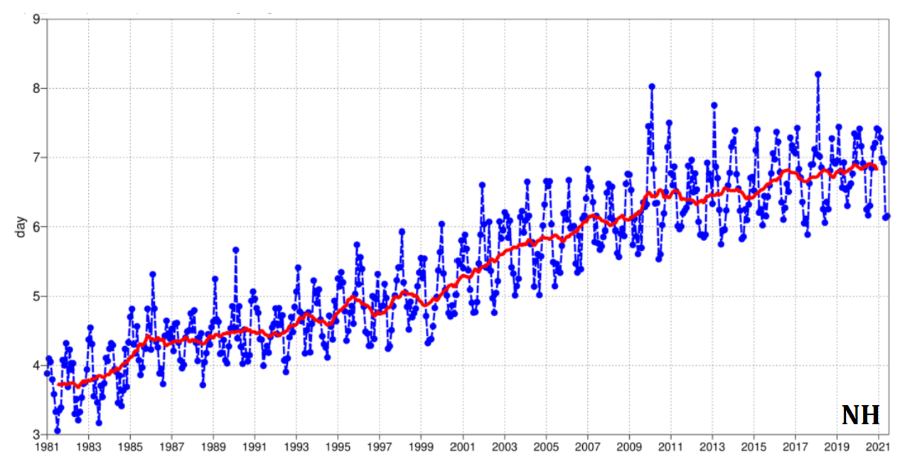
To date, weather forecasts are based on numerical weather prediction: numerical integration of partial differential equations (PDEs) describing atmospheric motion from measured initial conditions. The equations governing weather have been researched since the early 1900s [Lynch, 2008], and numerically solving these PDEs was an early success of computers [Charney, 1952]. Steady improvements in forecasting accuracy have been made, including improved data, data assimilation, and numerical methods (Figure 1).

There’s a pretty remarkable dataset available in the realm of AI for science: the ERA5 global reanalysis dataset, which contains hourly estimates of numerous 3D atmospheric, land, and ocean features at a horizontal resolution of 30 km over the past 80 years. This dataset was synthesized from up to 25M-per-day measurements from Earth-observing satellites and weather stations. Can machine learning be used to learn to forecast the weather better, either by more efficiently/effectively solving the weather PDEs or by learning a better model?
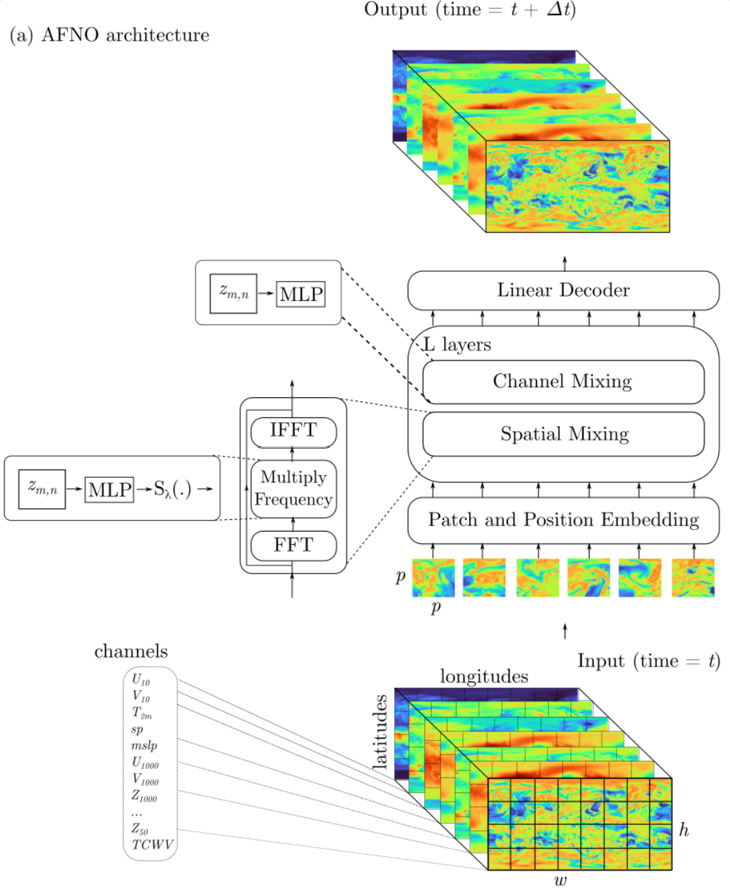
The FourCastNet paper [Pathak, 2022] trains an Adaptive Fourier Neural Operator (AFNO) network [Guibas, 2022] to predict a collection of atmospheric variables at the next time step (6 hours into the future) given the current readout for those variables. The AFNO is an interesting choice here: it takes inspiration from both neural operators, which were originally designed to efficiently solve PDEs, and Vision Transformers (ViT), which can learn complex functions from large image datasets. This choice seems to have been motivated by several factors: (i) We know that weather is well-modeled by PDEs, (ii) the ERA5 dataset can be represented as images where each pixel location corresponds to a \(.25^\circ \times .25^\circ\) latitude/longitude region, and each channel corresponds to a different atmospheric variable. So, maybe some amalgam of neural operators and transformers is a feasible choice to capture the nature of this data. Moreover, AFNO promises to combine computational efficiency (i.e., low computational complexity) with a comparably low memory footprint.

Training
One of the issues with almost every temporal process is that it has multiple time scales that we want to model. To predict the weather \(k\) time points into the future, FourCastNet must be run iteratively \(k\) times, and errors can accumulate so that inputs are out-of-domain. So, instead of training on the full temporal resolution of the data, FourCastNet is trained at 6-hour resolution. Probably badness would happen if it was trained at 1-hour resolution, and then run iteratively \(6\cdot k\) times. Interestingly, they first train on 6-hour predictions, then fine-tune to minimize 12-hour prediction errors when calling the network twice recursively.
Evaluation
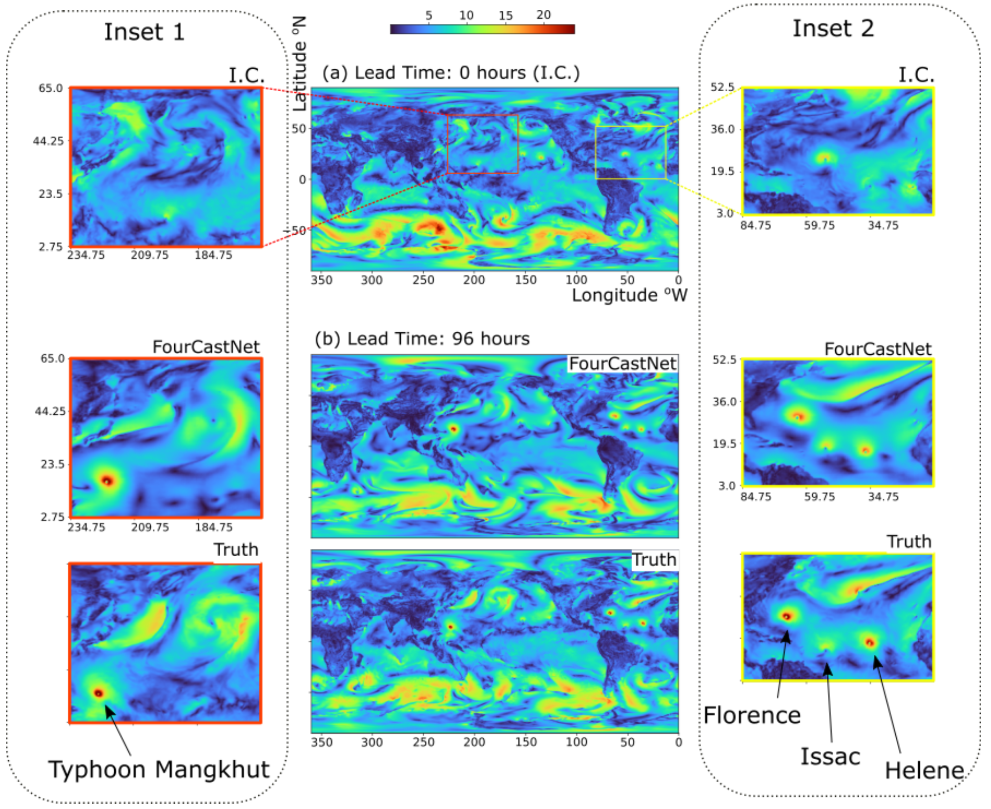
Most of the paper is devoted to evaluating the performance of the weather forecasts. They show that their predictions are qualitatively accurate on predicting the formation and trajectory of a cyclone and hurricane, as well as patterns of an atmospheric river within the range of 2–4 days. They quantitatively compare the accuracy of the FourCastNet prediction to the ECMWF’s physics-based Integrated Forecasting System (IFS). Accuracy is worse (with a few exceptions), but comparable. For comparison, more recent ML-based models, including GraphCast [Lam, 2023] and GenCast [Price, 2024] report superior performance to ECMWF.

The improvement stressed in this work is computational, particularly when predicting an ensemble of forecasts. Here, they add Gaussian noise to the initial observations and produce slightly different forecasts to estimate the distribution. While the IFS forecast takes minutes on a giant supercomputing cluster, FourCastNet’s forecast takes 7 seconds on 4 A100s. There’s a bit of apples to oranges in this comparison, both in terms of the problem and the type of computers when reporting just how much more efficient their approach is, but it is unquestionably more efficient. Computational efficiency is also the major improvement that neural operators offer over classical methods for solving PDEs.
Thoughts
One closing question is how ML solves this problem: Is it learning to model the weather in the same way that the governing physics equations do? Or is it more about learning what initial conditions are similar and memorizing? In some ways, memorization seems like it may be a step backwards—before numerical weather prediction was a thing, meteorologists did something closer to memorization:
Richardson’s book opens with a discussion of then-current practice in the Meteorological Office. He describes the use of an Index of Weather Maps, constructed by classifying old synoptic charts into categories. The Index assisted the forecaster to find previous maps resembling the current one and therewith to deduce the likely development by studying the evolution of these earlier cases. But Richardson was not optimistic about this method. He wrote that “The forecast is based on the supposition that what the atmosphere did then, it will do again now. […] The past history of the atmosphere is used, so to speak, as a full-scale working model of its present self”. […] the Nautical Almanac, that marvel of accurate forecasting, is not based on the principle that astronomical history repeats itself in the aggregate. It would be safe to say that a particular disposition of stars, planets and satellites never occurs twice. Why then should we expect a present weather map to be exactly represented in a catalogue of past weather?
— From [Lynch, 2008]
Things we are taking away from this paper:
- ERA 5 is a cool dataset!
- It’s going to allow ML to beat physics at weather forecasting, with lots of caveats about the classical work that goes into assimilating raw observations into these nicely gridded measurements, and probably lots of things we don’t understand about weather. Will there be noticeable improvements to us in our weather forecasts soon??
- There’s a lot of work to do on the details of what data is used, what is predicted, and how it is evaluated. We were happy to see that the ECMWF now has an experimental AIFS—the Artificial Intelligence/Integrated Forecasting System. They’ve released implementations of several of the SOTA models that you can get with
pip install ai-models - AFNO is an interesting choice because of (a) its connection to PDEs that underly many processes we want to model and (b) computational efficiency. There are also open-source implementations of AFNO and FourCastNet, and a FourCastNet colab notebook
About the AFNO
We spent some time trying to understand the AFNO, and its relationship to both neural operators and vision transformers. A stated goal of the AFNO is to capture important properties of a transformer, but reduce the memory and computational requirements to not depend on the context length / number of image patches squared. This is important in the FourCastNet context, as each weather image each image is divided into \(h\times w = 720 \times 1440\) patches of size \(8\times 8\), i.e., each image has \(720/8 \cdot 1440/8 = 16,200\) patches.
Each AFNO block does the following:
- Let \(X \in \mathcal{R}^{h \times w \times d}\) be the input, where \(N=hw\) is the length of the token sequence, and \(d\) is the token embedding dimension.
- Use the patch location \((m,n)\) to convert to frequency space: \[z_{uv} = [\textrm{DFT}(X)]_{uv} = \frac{1}{\sqrt{mn}} \sum_{mn} x_{mn} \exp( - 2\pi i (um/h+vn/w) ).\] This can be viewed as token mixing, creating direct connections between every input spatial token \(x_{mn}\) and frequency token \(z_{uv}\).
- In the frequency space, channels are adaptively mixed through 2-layer MLPs: \[\tilde{z}_{uv} = \text{BlockMLP}(z_{uv}) = W_2 \sigma( W_1 z_{uv} )\] where \(W_1, W_2 \in \mathcal{R}^{d \times d}\) are learned block-diagonal matrices. Note that this is described as part of the “spatial mixing” of AFNO, even though, as far as we can tell, it only mixes across channels.
- As natural images are inherently sparse in the frequency domain, sparsity can be encouraged by applying \[S_{\lambda}(\tilde{z}_{uv}) := \textrm{sign}(\tilde{z}_{uv})\max(|\tilde{z}_{uv}|-\lambda,0),\] where the parameter \(\lambda\) controls the sparsity.
- Demix tokens with the inverse Fourier transform: \[y_{mn} = [\textrm{IDFT}(\tilde{Z})]_{mn} = \frac{1}{\sqrt{mn}} \sum_{uv} \tilde{z}_{uv} \exp( 2 \pi i (um/h+vn/w) )\]
- Perform another two-layer MLP to mix across channels in the spatial domain: \[\tilde{y}_{mn} = \text{BlockMLP}(y_{mn})\] This step is not mentioned, as far as we can tell, in the text of the AFNO paper, but is in Figure 2 and the AFNO code base. It is referred to as channel mixing.
Like the MLP mixer, its relationship to the transformer is most obviously that there is some mixing across tokens and mixing across channels. As we understand it, mixing across tokens happens through the Fourier transforms, and thus is not learned or input-dependent, but there are direct connections between all tokens.
The AFNO paper also shows that a self-attention layer \[ \textrm{Att}(X) = \text{softmax}( XW_q(X W_k)^\top / \sqrt{d} ) X W_v \] can (ish) be expressed as a kernel integral: \[ \textrm{Att}(X)[s] = \sum_t X[t] \kappa(s,t), \] with \[\kappa(s,t) = \text{softmax}( XW_q(X W_k)^\top / \sqrt{d} ) W_v\,.\] Note that here \(\kappa\) is a kernel that depends on \(X[t]\). (Also note that \(X[t]\) is a notation convenience, assigning a linear index to each token \(x_{mn}\) with \(s,t \in [hw]\), i.e., \(X[t] := X[n_t,m_t]\)). Viewing \(X\) as a function on the continuous space \(D \subset \mathcal{R}^2\) instead of as a matrix with values at discrete indices, they write this sum as an integral: \[\mathcal{K}(X)(s) = \int_D \kappa(s,t) X(t).\] If we now let \(\kappa\) depend only on the distance between \(s\) and \(t\), i.e., \(\kappa(s,t) = \kappa(s-t)\), then it becomes shift-invariant (which is not generally the case), and we can compute the convolution integral as multiplication in the Fourier domain: \[\mathcal{K}(X)(s) = \mathcal{F}^{-1}( \mathcal{F}(\kappa) \cdot \mathcal{F}(X))(s).\] There is a somewhat non-straightforward relationship between these equations and the steps of the AFNO. In AFNO, the multiplication is realized by the 2-layer MLP \(\tilde{z}_{uv} = W_2 \sigma( W_1 z_{uv} )\). If one wants to write this as multiplication with the Fourier transform \(g\) of a kernel, this becomes \(\tilde{z}_{uv} = W_2 \sigma( W_1 z_{uv} ) =: g(z_{uv}) z_{uv}\), where the kernel depends on \(z_{uv}\) and, hence, on \(X\). The reduction in complexity compared to transformers comes from the fact that the weights \(W_1, W_2\) here are shared for all tokens.
References
[Pathak, 2022] Jaideep Pathak, Shashank Subramanian, Peter Harrington, Sanjeev Raja, Ashesh Chattopadhyay, Morteza Mardani, Thorsten Kurth, David Hall, Zongyi Li, Kamyar Azizzadenesheli, Pedram Hassanzadeh, Karthik Kashinath, and Animashree Anandkumar, “FourCastNet: A Global Data-driven High-resolution Weather Model using Adaptive Fourier Neural Operators”, 2022. 🔗
[Lynch, 2008] Peter Lynch, “The origins of computer weather prediction and climate modeling”, 2008. 🔗
[Charney, 1952] J. G. Charney, R. Fjortoft, & J. Von Neumann, “Numerical integration of the barotropic vorticity equation”, 1952. 🔗
[Haiden, 2021] T. Haiden, M. Janousek, F. Vitart, Z. Ben Bouallegue, L. Ferranti, F. Prates, and D. Richardson, “Evaluation of ECMWF forecasts, including the 2021 upgrade”, 2021. 🔗
[Guibas, 2022] John Guibas, Morteza Mardani, Zongyi Li, Andrew Tao, Anima Anandkumar, Bryan Catanzaro, “Adaptive Fourier Neural Operators: Efficient Token Mixers for Transformers”, 2022. 🔗
[Lam, 2023] Remi Lam, Alvaro Sanchez-Gonzalez, Matthew Willson, Peter Wirnsberger, Meire Fortunato, Ferran Alet, Suman Ravuri, Timo Ewalds, Zach Eaton-Rosen, Weihua Hu, Alexander Merose, Stephan Hoyer, George Holland, Oriol Vinyals, Jacklynn Stott, Alexander Pritzel, Shakir Mohamed, and Peter Battaglia, “GraphCast: Learning skillful medium-range global weather forecasting”, 2023. 🔗
[Price, 2024] Ilan Price, Alvaro Sanchez-Gonzalez, Ferran Alet, Tom R. Andersson, Andrew El-Kadi, Dominic Masters, Timo Ewalds, Jacklynn Stott, Shakir Mohamed, Peter Battaglia, Remi Lam and Matthew Willson, “GenCast: Diffusion-based ensemble forecasting for medium-range weather”, 2024. 🔗